

Parallel SNP identification
by Ketil Malde; March 26, 2014
Basics
Lately, I’ve been trying to do SNP identification. Basically, we take samples from different populations (geographically separated, or based on some phenotype or property), sequence them in pools, and then we want to identify variants that are more specific to certain populations. The basic method is to map sequences to a reference genome, and examine the sites where the mappings disagree - either with the reference, or with each other.
There are many different implementation of this, most require indiviual genotypes (that is, each position is identified for each individual as homo- or heterozygotic), and most are geared towards finding variant positions, rather than finding diagnostic variants. Many methods - at least those I’ve tested are also quite slow, and they give output that is harder to use (i.e. pairwise scores, rather than overall).
In my case, we have pooled sequences (i.e. not individual data), we want diagnostic variants (i.e. those that differ most between populations), and we only need candidates that will be tested on individuals later, so some errors are okay. So I implemented my own tool for this, and ..uh.. invented some new measures for estimating diversity. (Yes, I know, I know. But on the other hand, it does look pretty good, in my brief testing I get less than a 0.06% FP positive rate - and plenty of true positives. But if things work out, you’ll hear more about that later.)
Parallel implementation
Anyway - my program is reasonably fast, but ‘samtools mpileup’ is a bit faster. So I thought I’d parallelize the execution. After all, we live in the age of multicore and functional programming, meaning plenty of CPUs, and an abundance of parallel programming paradigms at our disposal. Since the program basically is a simple function applied line by line, it should be easy to parallelize with ‘parMap’ or something similarly straightforward. The probelm with ‘parMap’ is that - although it gets a speedup for short inputs - it builds a list with one MVar per input (or IVars if you use the [Par monad]) strictly. So for my input - three billion records or so - this will be quite impractical.
After toying a bit with different modeles, I ended up used a rather quick and dirty hack. Avert your eyes, or suffer the consequences:
parMap :: (b -> a) -> [b] -> IO [a]
parMap f xs = do
  outs <- replicateM t newEmptyMVar
  ins  <- replicateM t newEmptyMVar
  sequence_ [forkIO (worker i o) | (i,o) <- zip ins outs]
  forkIO $ sequence_ [putMVar i (f x) | (i,x) <- zip (cycle ins) xs]
  sequence' [takeMVar o | (o,_) <- zip (cycle outs) xs]

worker :: MVar a -> MVar a -> IO b
worker imv omv = forever $ do
  ex <- takeMVar imv
  ex `seq` putMVar omv ex
Basically, I use worker threads with two MVars for input and output, arranged in circular queues. The input MVars are populated by a separate thread, and then the outputs are collected in sequence. I don’t bother about terminating threads or cleaning up, so it’s likely this would leak space or have other problems. But it seems to work okay for my purposes. And sequence_ is the normal sequence, but lazy, i.e. it uses unsafeInterleaveIO to delay execution.
Benchmarks
To test the parallel performance, I first ran samtools mpileup on six BAM files, and then extracted the first ten million records (lines) from the output file. I then processed the result, calculating confidence intervals, a chi-squared test, and Fst, with the results in the table below.
| Threads | wall time | time (s) | size (MB) | cpu (s) | sys (s) |
|---|---|---|---|---|---|
| 1 | 8:00 | 480 | 32.0 | 472 | 7 |
| 2 | 4:40 | 280 | 39.7 | 525 | 19 |
| 4 | 2:33 | 153 | 40.1 | 550 | 32 |
| 8 | 1:43 | 103 | 40.7 | 689 | 57 |
| 12 | 1:50 | 110 | 36.9 | 978 | 106 |
| 16 | 1:33 | 93 | 40.3 | 1047 | 125 |
| 24 | 1:17 | 77 | 40.7 | 1231 | 152 |
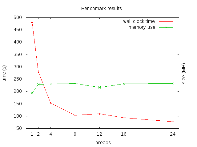
Benchmark results for different numbers of threads.
I would guess that system time is Linux scheduling overhead.
I thought the time with 12 threads was a fluke, but then I reran it thrice: 1:52, 1:50, 1:52. Strange? The only explanation I can see, is that the machine has 12 real cores (hyperthreading giving the pretense of 24), and that running the same number of threads gives some undesirable effect. Running for t={10,11,13,14} gives
| Threads | time |
|---|---|
| 10 | 1:45 |
| 11 | 1:44 |
| 12 | 1:51 |
| 13 | 1:45 |
| 14 | 1:45 |
So: apparently a fluke in the middle there, and 11 seems like a local minimum. So let’s try also with 23 threads:
% /usr/bin/time varan 10m.mpile.out --conf --chi --f-st > /dev/null +RTS -N23
1165.14user 137.80system 1:15.10elapsed 1734%CPU (0avgtext+0avgdata 41364maxresident)k
0inputs+0outputs (0major+10518minor)pagefaults 0swaps
Sure enough, slightly faster than 24, and 5% less work overall. Of course, the GHC scheduler is constantly being improved, so this will likely change. These numbers were with 7.6.3, I also have a 32-core machine with 7.0.4, but currently, that refuses to compile some of the dependencies.
Conclusions
Memory stays roughly constant (and quite low), scalability is okay, but starts to suffer with increasing parallelism, and gains are small beyond about eight threads.
Genomes vary enourmously in size, from a handful of megabases to multiple gigabases (each position corresponding to a record here), but scaling this up to human-sized genomes at about three gigabases indicates a processing time of roughly two days for a single-threaded run, reduced to about ten hours if you can throw four CPUs at it. This particular difference is important, as you can start the job as you leave work, and have the results ready the next morning (as opposed to waiting to over the weekend). Anyway, the bottleneck is now samtools. I can live with that.
